This page contains guidelines for observing with Hector. As with all instrument systems, things will change from run to run, so always check here before you go observing.
Equally, a document such as this will never cover everything exactly or predict all changes at the telescope. Please use this document as a guideline and always check and test things as you go.
The Night before the first observing night………………………………………………. 2
The First Night…………………………………………………………………………………………… 3
Before Sunset Essentials…………………………………………………………………………… 3
Initial Hardware Set-up AAOmega………………………………………………………… 4
Initial Hardware Set-up Spector……………………………………………………………. 4
Initial Software Set-up…………………………………………………………………………… 4
Instrument Control Software…………………………………………………………….. 5
Default Observing Procedure…………………………………………………………………… 8
Logs *** update ***……………………………………………………………………………… 8
Plate Plugging………………………………………………………………………………………… 8
Hexabundle Designations………………………………………………………………….. 8
Changing the Plate…………………………………………………………………………… 10
Updating and Loading the Hector Configuration File…………………….. 13
Focusing the Spectrographs……………………………………………………………….. 14
Data Reduction with 2dfdr and the Hector Software…………………………. 15
Data reduction machine at AAT………………………………………………………. 15
First Night Essential: check 2dfdr…………………………………………………….. 15
First Night Essential: check the Hector package………………………………… 16
Load the observed frames to the data reduction machine……………. 17
Disable and enable files…………………………………………………………………… 18
Summary: data reduction at AAT…………………………………………………….. 19
Tips: reduce subsamples and re-reduce frames…………………………….. 19
Essential: check tramline mapping with check_tramline()……………… 20
Essential: quick-look plots to check centring………………………………….. 21
Essential: QC summary……………………………………………………………………. 24
Essential: upload raw data to the data central cloud……………………… 25
Essential: upload log on the Hector wiki…………………………………………. 26
Night-time Calibration Frames (Flats, Arcs, Twilights)………………………… 26
Focussing the Telescope…………………………………………………………………………. 28
Measuring and Correcting the Global Plate Rotation……………………………. 28
Spectrophotometric Standards………………………………………………………………. 29
Observing Galaxies…………………………………………………………………………………. 32
Day-time Calibrations (Biases, Darks and Long-slit Flats)……………………… 34
Biases and Darks…………………………………………………………………………………. 34
Long-slit Flats……………………………………………………………………………………….. 34
Drama (Hector control software Failure)……………………………………………….. 35
At the End of the Night……………………………………………………………………………. 36
The Night before the first observing night
The Hector robot should be used to configure the first two plates for the run.
Details of running the Hector robot are given in the Hector Robot Instructions.
The robot and tile files for the run will be sent out in the week before the run and can be downloaded from data central.
The robot pc is intentionally not online to the world and therefore the web browser cannot be used to download the files from Data Central.
To copy the files to the robot use aatlxe, aatlxh or aatliu on the Hector account to download the files, then copy them to the /hectorrobot/transfer directory.
On aatliu, the aatinst user can manipulate files in /hectorrobot/transfer
On aatlxe and aatlxh the hector user can manipulate files in /hectorrobot/transfer
This directory maps to c:\transfer on the hector robot PC itself.
Users other than those specified above can read the transfer directory but can not place or change files there. The aatinst account on aatliu and the hector account on aatlxe are the accounts that will always be used for hector observing.
Download the git python software to aatlxe or aatlxh for data reduction etc.
The First Night
NOTE that Hector observers are required to have the first plate plugged before 4pm ready to focus the spectrographs ahead of taking twilights. Even if the forecast looks like solid cloud, at least one Hector observer must stay up until within 60 mins before twilight ever night. If it is solid cloud and not looking like clearing by 60 mins before twilight then there may not be time to get a full exposure if it does clear. Do not assume the weather will not clear as Siding Spring weather continues to surprise us! If it is clear then observers stay up to take morning twilights just before sunrise.
Before Sunset Essentials
- The instrument will be installed by site staff starting around 08:00, observers are not specifically required for that instrument change.
- BEFORE the site staff leave at 4pm, take a flat to ensure the tramlines are all on the AAOmega detector. FIRST the pistons for the top and bottom sky fibre on AAOmega must be moved to position 1, 2 or 3 to see light in the dome. Those two pistons are marked with a silver dot on the subplate lid above that piston and are A3-1 and A2-7. Take image with dome lights on (short exposure) using the flap flat (fibre flat, 75W AAOmega lamp), dummy, 1 sec. Check all four corners of the image to ensure the tramlines are on the detector. If any of the tramlines are at the very edge of the detector such that they would not be able to be fit, ask site staff to adjust the mounting of the slit on AAOmega until the tramlines are all on the detector. When doing this test, make sure that the gratings are at the correct angles/wavelengths for Hector observations. Changes in the grating/camera angle can move the tramlines.
- Observers should gather in the control room at 15:00 (seasonal) for a “Hector huddle” to ensure the observing plan is clear to all. You will need to meet earlier if a plate needs to be configured for the start of the night.
- The first two field plates for the night should be put on to configure as early as possible. At 14:00 the observers should start the robot configuring the first plate so that it is configured in time to be installed and plugged before the start of calibrations at 16:00. As soon as the first plate is configured, the second plate should be put on to the positioner to be configured.
*** The following should go elsewhere, not essential here *** At the end of the first (and subsequent) nights, before going to bed, the first field for the following night should be started configuring on the robot. - Hardware testing, including plugging, should be finished by 16:00 when dome lights are turned off and you can start taking frames.
- Use the time between 16:00 and twilight to take and reduce a near-zenith dome flat and arc. Run them through the data reduction to check all the software is working. These frames are necessary for quick reductions of the first night-time data. Note that the new flat field screen does not get to zenith, so take a near-zenith flat.
- All systems, including the robot and control and reduction software, should be tested well advance of twilight.
Initial Hardware Set-up AAOmega
AAT technical staff will install Hector on the 2dF top end of the AAT.
Spector has no parts that need to be interacted with by astronomers – Do not go into the Spector room, it is thermally controlled. There are no dark slides on Spector (it uses an aperture instead) and no gratings to change.
IMPORTANT The Hector slit block on AAOmega attaches to the rotating slit exchange mount on AAOmega. It MUST NOT be rotated while Hector is attached. Therefore, DO NOT ATTEMPT TO MOVE THE SLIT BLOCK.
Very rarely the drama software and the spectrograph can get confused about which slit is in position and you must tell it that the Hector-AAOmega slit is in. In the drama software the correct slit position may still be called SAMI . To tell AAOmega that SAMI (or SLIT3) is in position type the following in a terminal on aatlxy.
ditscmd -s SPECTRO@aaomegaserver SLIT 3
Once Hector has been installed, check that the correct gratings and dichroic are installed in AAOmega and that they are all uncovered. If any need to be changed, ask the site staff to do it or to help you. Do not do this by yourself unless you know what you are doing – optics are very heavy (especially the dichroic).
For survey operations we use:
- Dichroic: 570nm
- Blue arm grating: 580V, central/blaze wavelength 4850A to cover 3700-5800A
- Red arm grating: 1000R, central/blaze wavelength 6830A to cover 6290-7400A
There can be an offset between the requested central wavelength and that returned by the spectrograph, so check that the wavelength coverage is correct by reducing an arc and checking that for all fibres the data covers the required range. Problems are most likely to be visible in the red (due to shorter wavelength coverage). In the red arm in particular, make sure that the 6300A line (in night sky and in galaxies, slightly redshifted) is within the wavelength range. Ideally the 6300A is just on the detector, which allows the red spectrograph to extend its coverage to just beyond the atmospheric absorption band at the red end of the spectrum.
Check with the site staff at the start of your run whether to use the right of left amplifier for AAOmega red CCD since there were issues with one or other amplifier at different times during the SAMI Survey.
Check that there is no evidence for frosting on the CCD in the blue camera (this has only been seen in the past in the blue). The blue camera has some contamination, which over time can deposit on the front face of the CCD. It requires warming and pumping to remove, which typically takes 24hrs or more. This should have been checked by site technical staff, but please be aware of the potential problem. The best way to check this is via a well illuminated arc frame. Frosting on the CCD will tend to cause a large scattered light component around the bright arc lines. This is also seen for the 5577A sky line. If this is seen, contact site staff immediately and look at the CCD to check for direct evidence of the frosting. It is mostly likely to occur around the edge of the detector.
Initial Hardware Set-up Spector
There is no hardware setup required by astronomers for Spector.
Initial Software Set-up
There are two software systems that you must set up, the control software and the hector python package.
Instrument Control Software
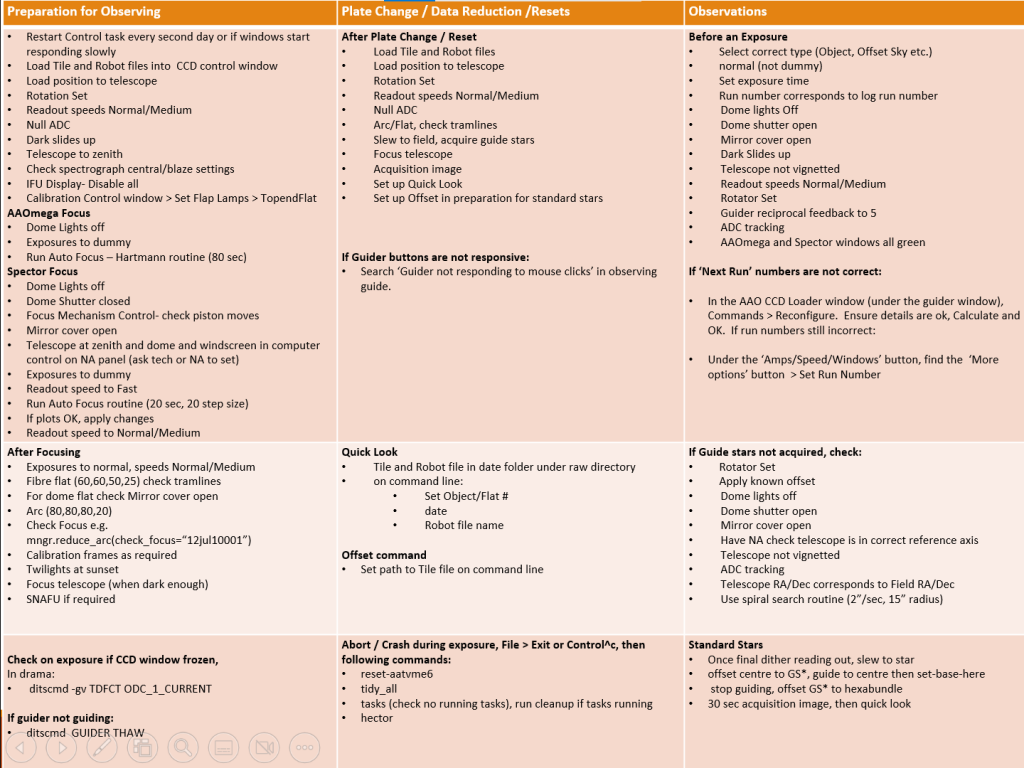
The main computer in the AAT control room has four screens and a number of dialogues boxes for controlling the instrument and telescope. The most important are described below.
The IFU control task
This dialogue box contains information about the status of the telescope and each spectrograph. From here, you can load the main CCD control task and the AAOmega and Spector control tasks by clicking on the “more” box below each heading.
The Control Room GUI layout
The main computer in the AAT control room has four screens and a number of dialogues boxes for controlling the instrument and telescope. The most important are described below.
The IFU control task
This dialogue box contains information about the status of the telescope and each spectrograph. From here, you can load the main CCD control task and the AAOmega and Spector control tasks by clicking on the “more” box below each heading.
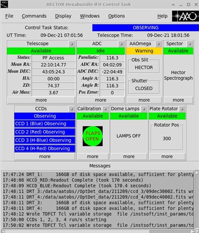
The CCD control task
The CCD control task is where you can take exposures. The 4 boxes at the top gives the status of each of the 4 CCDs (AAOmega blue, AAOmega red, Spector blue and Spector red). These should be coloured green if everything is healthy. The boxes below which say ‘Idle’ will change during an exposure. Whilst exposing, they will fill up with a green bar and state the remaining exposure time. Whilst reading out this bar will turn cyan.
The various different exposure types are listed on the left, with ‘Dark’ currently selected. These different options will be explained below. The exposure time for each CCD is set on the right, next to the boxes reading ‘BL’, ‘RD’, ‘HBL’, ‘HRD’.
IMPORTANT. The AAOmega GUI contains several buttons allowing the user to set the “observation type” of any exposed file. This is saved in the header of the file as the OBSTYPE keyword. You must select the correct type for each file you observe. We DO NOT use all available options.
| Button Name | OBSTYPE Keyword Value | Exposures we use it for |
| “Object” | MFOBJECT | Any astrophysical object, including standard stars |
| “Dark” | DARK | Dark frames |
| “Bias” | BIAS | Bias frames |
| “Offset Sky” | MFSKY | Twilight flats |
| “Twilight flat (previously Offset Flat)” | SFLAT | Do not use! EVER. |
| “Detector Flat” | DFLAT | Long-slit flats |
| “Fibre Flat” | MFFFF | Any fibre flat field – whether flap or dome |
| “Arc” | MFARC | Arc frames |
| “Flux Cal” | MFFLX | Do not use! EVER. |
A “Dome” tab is available in the Control Task “Telescope” dialog . The dome will automatically slew into position when a dome flat exposure is begun. It will first check that the dome can reach the position.
New status lines in the “Telescope” dialog show if the dome is slewing etc, if it is in the flat field position and the dome error (which is useful to get a feel of how long it will take to get to position).
Default Observing Procedure
Logs *** update ***
The logs will be kept in online form so the csv files can be merged into a database of observations.
Plate Plugging
After the initial set-up is done on the first night, and first thing on all subsequent nights, you will “plug” the first plate of the night, either be a star plate or a galaxy plate. There are 19 galaxy hexabundles, 2 star hexabundles, and 6 guide bundles plus sky fibres to be positioned.
Hexabundle Designations
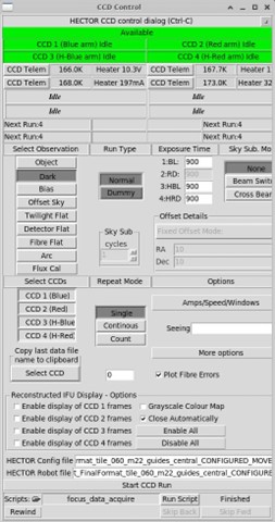
The Hector hexabundles have a hexabundle letter written on the bundle. The hexas appear in a certain order in the AAOmega and Spector slit (the slit position) and on the readout screen in the control room. The slit position 1 is positioned at the top of the slit and the top of the readout screen.
The hexabundles are arranged on the slit like so:
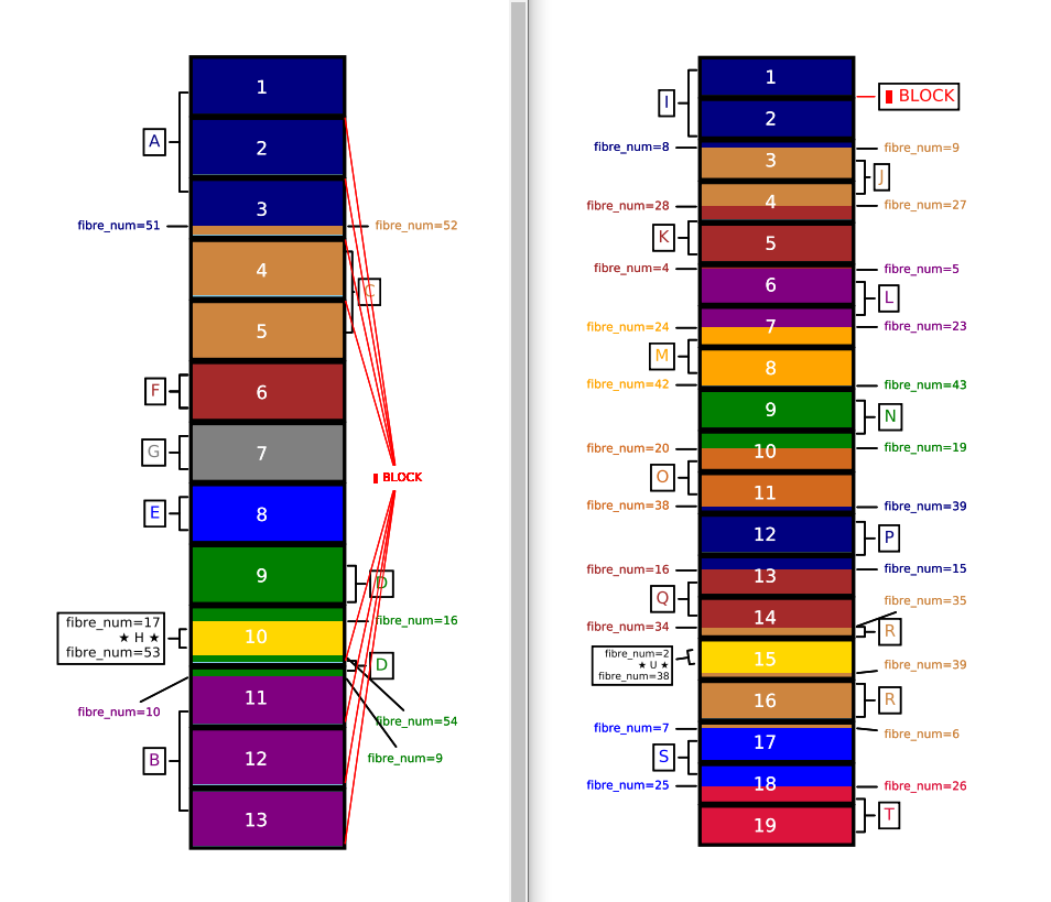
Fig. Graphic of the slitlets in order from top to bottom of screen and where the fibres for each hexabundle sit on the slitlets. AAOmega on right with 13 slitlets and Spector on left with 19 slitlets.
- AAOmega has 13 slitlets as labelled with numbers with 63 fibres on each slitlet.
- Spector has 19 slitlets as labelled with numbers with 45 fibres on each slitlet.
- The positions on slitlets which are not occupied are labelled as ‘BLOCK’ in red text and will appear as gaps on the detector. These are fibres that were left intentionally not connected to a hexabundle or sky because the SAMI experience showed that wider gaps were required between slitlets for calibration. NOTE that these are fibres that are permanently BLOCKED. However the gaps will be widened further on tiles when a sky fibre adjacent to the gap is required to be blocked off due to contamination, and the fibre mapping will list BLOCK-Sky, but they will not be shown on this static plot (see below for plot showing changing sky shuffled fibres).
- The hexabundles on stars are labelled in black with star symbol inside a box with starting and ending fibre numbers.
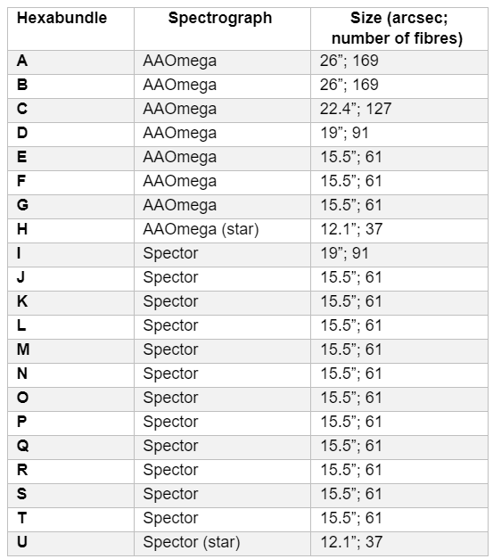
- Each hexabundle A to U is shown in a different colour block and the slitlets covering the same hexabundle are shaded accordingly with the starting and ending fibre numbers labelled. The following table lists the hexabundle and their letters have corresponding labels to the sides of the slitlet graphic.
TABLE: Hexabundles
Changing the Plate
To change a plate, you must be a trained plugger. If you notice anything wrong, unusual, broken or unsure when doing the plate change then contact Julia Bryant immediately on Julia.bryant@sydney.edu.au or 0432951638. Continuing with damaged parts may destroy other parts or prevent those parts from being saved.
The steps are as follows:-
- Ask for the telescope to be brought to prime focus access, confirm with the telescope operator that the telescope is in manual mode, and then tag the telescope at the control console so everyone knows you are working in the dome. Due to complaints from other telescopes on the mountain, the dome lights CAN NOT be put on during plate plugging when the dome is open – instead use the lamp at prime focus access and/or the SAMI head torch.
- The next plate to go on the telescope should be sitting in the robot plate holder as it would have been configured prior, or during the observing of the plate that is on the telescope.
- Unplug the hexabundles from the magnets on the plate that is on the top end and put each one in a holder position:
- Unplugging should be done with the plugging tool.
- IT IS ESSENTIAL that the magnets are not accidentally moved while plugging and unplugging the hexabundles or it will cause them to not be in the right position for the robot to pick up and that will crash the pick up arm into the magnet and destroy the magnet.
- IF a magnet is accidentally bumped then the recovery procedure must be followed (details below). This procedure removes the magnet manually from the plate and runs the recovery code on the robot to put the magnet back in a position known to the robot.
- The hexabundles are incredibly sensitive to shocks because the tiny 3mm prism is bonded to a cantilevered 2mm of glass. The nature of a glass-to-glass bond with highly polished glass means that a shock will cause a fracture to propagate between the two glass surfaces and the prism will come off, destroying the ability to use the hexabundle. Therefore ALL CARE MUST BE TAKEN NOT TO SHOCK, JOLT, or KNOCK the hexabundles on anything.
- As the hexabundles are put into the holders on either side of the top end holder, a rod should be moved across the holes in the holders to ensure the hexabundle and guide bundles cannot be accidentally pulled out of those holders by snagging.
- Once all hexabundles and guide bundles are in the holders, then the sky fibres must be moved out of the way before removing the plate:
- The sky fibres are each in individual pistons with fragile prisms glued on (same risks as for the hexabundle prisms above). The pistons are arranged in subplates. The Subplates feeding AAOmega (A1-A5) have 7 pistons per subplate and those feeding Spector have 8 pistons.
- The subplates are arranged around the field plate as seen from prime focus access according to the graphic below.
- Each piston can be moved to one of 4 positions:
0 – blocked off – no light will get to the fibre – used when contaminated with an object
1, 2, 3 – Three different positions – the code has selected a position that will not be contaminated by star light.
There is a fifth, fake position between 0 and 1 which lines up with the screw holes and is not used.
- When changing the field plate, the sky fibre pistons must be in position 1 or 0 to avoid interference with the plate. Move all pistons back to 1 or 0 before removing the field plate.
- Attach the plate holder to the plate.
- Loosen the three plate holding tabs using the torque wrench.
- Lift the plate out of the top end carefully moving straight upwards from the locator pins.
- Put the plate aside on the table.
- Transfer the plate holder to the newly configured plate on the robot plate holder.
- Lift that plate directly upwards off the locator pins and out of the robot enclosure.
- Put the plate into the top end and tighten the plate holder tabs. NOTE THESE tabs have sensors that will not allow the barrel to rotate if the plate holder tabs are not in position (otherwise the top end field lens and all of the fibres and hexabundles would be destroyed if it fell out when the top end tumbled).
- Plug the hexabundles and guide bundles from the holders onto the field plates matching the diagram for the field to be observed [more detail to be added here]. Positioning of the hexabundles on the field plate and the locations required for each of the sky fibre pistons in each subplate is shown in a plot like this one, which is generated for every field. East is to the right and North is down.
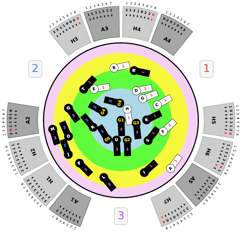
- The field plate is represented by the circle with 4 different zones represented by circular annuli. Those annuli are the different telecentricity zones with different magnet tilts in each zone. From inner to outer are zones 1 Blue, 2 Green, 3 Yellow, 4 Magenta. Note the circular magnets are labelled with numbers 1-4 for the zone they belong to, with numbering of the form Z-XX where Z is 1-4 for the zone and XX is the individual serial number of the circular magnet.
- Each hexabundle sits on a pair of magnets – one circular and one rectangular. The circular magnet centres the hexabundle on the galaxy and the rectangular magnet holds the “rotation arrestor” which set the rotation of the hexabundle on-sky. For each magnet pair and hence hexabundle placement, there is a circle+rectangle symbol on the plot, indicating the magnet pair to place each hexabundle on.
- Hexabundles are given letter names from A to U, with A to H feeding AAOmega and I to U feeding Spector. The hexabundle details are in the table “Hexabundles” above. The letter for the hexabundle that must be put on a given magnet pair is shown in the hexabundle plate file for each plate to be configured.
- AAOmega hexabundles represented by magnets labelled with black text in a white background.
- Spector hexabundles represented by magnets labelled with white text in a black background.
- Guide probes numbers 1 to 6 are represented by magnets labelled with yellow text in a black background.
- Hexabundles that have 37 cores and are designed to observe stars – one of each type AAOmega (hexa H) and Spector (hexa U).
- Sky fibre subplates are represented with wedge shapes surrounding the field plate with light and dark grey shades- ‘A’ numbered plates A1-A5 in dark grey feed the AAOMega spectrograph and ‘H’ numbered plates H1-H7 in light grey feed the Spector spectrograph.
- Set the sky fibres into position: Each sky fibre subplate contains pistons that set the location of the sky fibre on-sky and are changed to a different position for each tile observed. The number of each piston within the subplates runs clockwise from 1-7 or 1-8 and is written outside the subplates. The number of the position that each piston must be set to is written on the subplate. Pistons can be in sky positions 1, 2 or 3 or can be blocked off in position 0 if all three sky positions are contaminated.
- NOTE some pistons are not in use and are marked with a blue circle sticker – these stay in position 0.
- The Sky subplates surrounding the central field plate are numbered A1-A5 for the sky fibres that feed to the AAOmega spectrograph and H1-H7 for the sky fibres that feed to the Spector spectrograph. The number of each piston within the subplates runs clockwise from 1-7 or 1-8 and is written outside the subplates. The number of the position that each piston must be set to is written in the plots on top of the grey box representing the subplate.
- Secure all loose cables with the tie-offs and the black stretch cloth [More info to be added here].
- Use the button on the white box to the lower right to undo the detent so the barrel can be manually rotated. Rotate the barrel so that the HECTOR PLATE GOES DOWNWARDS and carefully watch for any cable snagging while rotating.
- Now set up the previous plate to be configured by the robot for the next field. Put the handle on the plate that was put aside and load it into the robot plate holder. Note that “up” on the telescope is “up” from the direction it is loaded into the plate holder.
- Lock the clamps on the plate holder.
- Check there are no unsecured magnet pieces or debris on the plate.
- Turn off the light and close the robot enclosure.
- Begin the plate loading process on the robot pc (either in the dome or remotely from the control room). [Full section to be added here which is the cheat sheet from the detailed robot control document. Add a link to the full robot document too.]
- Refocus the telescope on the acquired guide stars (see below on how to do this).
Updating and Loading the Hector Configuration File
For each observation, both a tile file and a robot file are required.
You will find the file on the wiki http://cloud.datacentral.org.au under Hector/Observing/<Run-dates>
The file names take the following example form:
Tile_A3667_T039.csv and
Robot_A3667_T039.csv
Upload both of the files into the Hector CCD Control Window, using the button at the bottom of the window. Once you have selected the correct file click Load Positions on the Telescope Control window.
IMPORTANT – Double check that you clicked the Load Positions from HECTOR File into Input Fields button!! This step is prone to human error.
You are now ready to observe this field, once night has fallen! (Or now if you are doing this in the middle of the night.)
Focusing the Spectrographs
Both the AAOmega and Spector spectrographs must be focused every afternoon when the dome is dark (after 16:00). Focus should not change much night to night, but on the first afternoon focusing may take about 20 minutes each spectrograph. As a starting point, use the focus positions for the last Hector run, which will be recorded in the online logs (and indicative values in this table). The AAOmega focus is done with an automatic Hartmann focus routine but the Spector spectrograph uses a contrast routine.
Starting point for focus values based on previous runs are (NOTE: the Spector values may substantially change if the piston mechanism has been homed):
| CCD Arm | Spatial Tilt | Spectral Tilt | Piston |
| AAOmega Blue | 1761 | 3435 | 87 |
| AAOmega Red | 871 | 2522 | 453 |
| Spector Blue | NA | NA | 2954 |
| Spector Red | NA | NA | 2343.01 |
AAOmega Procedure
- Before starting the focusing procedure set the file type to be dummy. These files will be saved but are not science files.
- For AAOmega:
- Click the “Auto Focus – Hartmann” button in the “AAOmega Spectrograph Control” (the flap should close automatically).
- A box will ask for the exposure time and a sensible value is 80 seconds.
- The software should switch the arc lamp on and off at the right times.
- The box will show (among other things) the current position of the focus values (the “Current H/W Position” row) and the suggested new settings. Compare these values. Click “Apply Arm” to the red and blue arms (or “Apply Both” at the bottom) to request the spectrograph to move to the suggested focus values.
- In an ideal world, the spectrograph focus values would then change to the desired values. This is not always the case, however, especially for the red arm! It is very important that you check that the current focus values match the suggested focus values after clicking “apply”. If they don’t, apply the values again until they do (or are at least very close).
- Repeat until the focus has converged (press ”Repeat”).
- Once the focus has converged it will show “Is the result in spec: Yes Yes Yes Yes Yes Yes”.
Spector
1. Focus must be redone every night. Twilight flats also require the spectrographs to be in focus.
2. Ensure the mirror cover is open before doing the focus as the focus routine uses the contrast method for Spector.
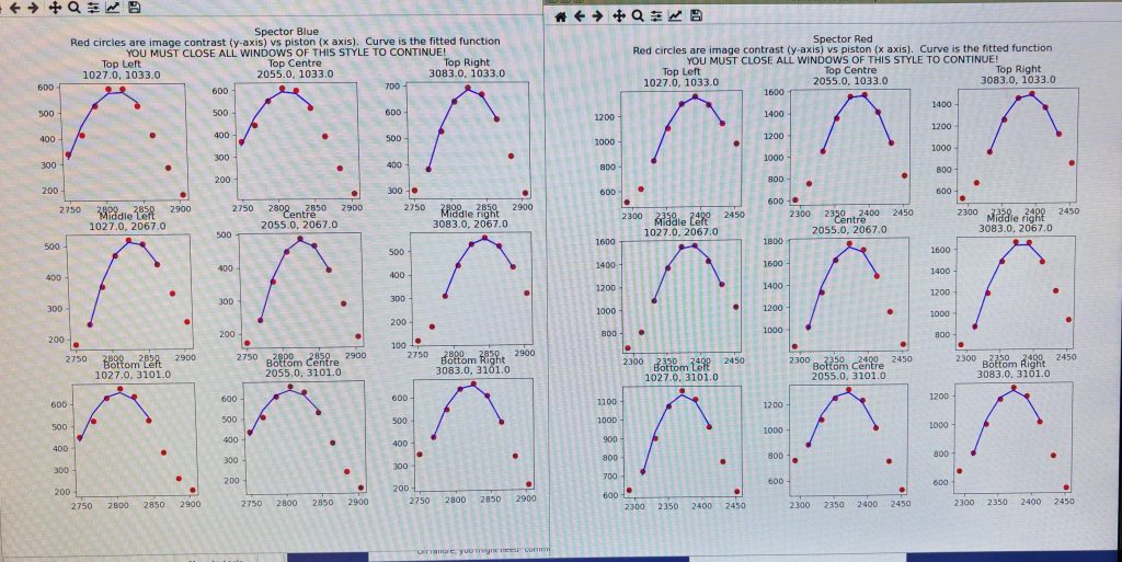
3. The focus curve must be symmetric or close to symmetric so that the peak is well constrained by points going a long way either side and not just one or two points on one side.
Spector Procedure
- Before running the Spector Auto Focus, open the Focus Mechanism Control window and attempt to move one of the pistons to a new position (make note of the original position so you can return the piston to this value). If the Requested position does not show in the Current position after selecting ‘Move’, then the Auto Focus routine will fail, as described in point 7 below. A Reset > Recover may solve this but generally a File > Exit of the Hector Control task is required before running the Auto Focus routine.
- Change readout speed to fast just for focussing – Don’t forget to change it back afterwards. To change readout speed, on the CCD Control window select ‘Amps/Speed/Windows’ and the speeds are listed for the two AAOmega then two Spector CCD. Only change the Spector CCDs but leave the AAOmega CCDs on normal (because they misbehave on fast).
- Open the Calibration window from the main Control task window. Select “set Flat Lamps” and select the Quartz_75_A lamp.[GU2] (This will instruct the below focus routine to use ‘flappy’ flats for focussing Spector).
- Click the “Auto Focus” button, and if the focus has no reason to have massively changed (e.g. if there had been work on the instrument) then select the “9 exposure mode”.
- A sensible exposure time is 20 sec.
- Select 20 as the size of the steps. (Larger values can go too far out of focus such that the fit is poor, but this value gives 4 points either side of focus within the intensity peak and should give a good fit.
- Once the plots appear, the system will not continue until you close both of the plot windows (one for each camera). The plots should show curves that are well fitted to the data and have a clear peak to the best intensity (I.e. best contrast where the best focus is). If the plots show no change in piston (I.e., a vertical column of different contrast values) then the focus routine will fail. From the Commands menu do reset recover (not by task!), then check the focus values in the Spector Control window are what they originally were– if not then use the focus mechanism control to drive them back to the best previously used focus values, then re-run the focus routine. [The reason this goes wrong is when the control software does not correctly read the focus position and thinks the focus position hasn’t changed. In the Spectrograph Control box the focus values will stay at the value they originally were rather than stepping through. By doing a Commands -> reset recover (not by task!) the software will correctly read the spectrograph positions and the focus routine should work].
- The Automatic Focus window shows a table of resulting values. (Note: The focus values will be given in the Control task window messages box as well). Only Piston is shown because that is the only value that can be adjusted for Spector. If the suggested values look acceptable then use the’Apply Both’ button to make the changes. Take note of the values then drive the CCD4 focus to 200 piston points LESS than the focussed value, and then drive it back to the focussed value (this is because it only reaches that focussed value when approached from the lower piston number side but the software approaches it from the wrong side – this will be changed in the routine soon, but for now do this extra manual step down and back in focus).
- Change the readout speed back to medium.
- Change “Quartz_75_A” to “top-end” (the main Control task window –> the Calibration window –> “set Flat Lamps” –> select “top-end”). This will allow observing scripts (i.e. “hector_dither” script) to default to using “dome flats”.
Data Reduction with 2dfdr and the Hector Software
Observers are requested to actively reduce data at the telescope. This enables the calibration frames to be checked and any data issues to be detected promptly. We also assess the quality (FWHM and transmission) of the object frames to decide whether any frames need to be retaken.
If you find any issues on the hector reduction package or the use of data reduction machine at AAT, please contact Sree Oh (sreemario@gmail.com), Madusha Gunawardhana (madusha.gunawardhana@sydney.edu.au), and cc Julia Bryant (julia.bryant@sydney.edu.au).
Data reduction machine at AAT
Find the machine labelled ‘DATA REDUCTION SYSTEM’ in the control room. The hector python package runs on aatlxe (preferred) or aatlxh. Log into either machine with the following username and password:
Username: hector
Password: RobotisGreat!
To set up the required terminals:
(base) hector@aatlxe:~$ ./setup_terminals.sh
First Night Essential: check 2dfdr
The first thing you should check is 2dfDR. Open a shell and try the following:
(base) hector@aatlxe:~$ drcontrol
It will pop up a window with Saturn. If not, please contact Sree Oh (sreemario@gmail.com) and Madusha Gunawardhana (madusha.gunawardhana@sydney.edu.au), immediately. If you do not get a response in time, you may install 2dfDR following the next step.
Not essential: Installing 2dfDR
Note: skip this step unless it is requested by the DR team
This section explains how to update the 2dfdr data deduction software on the Data Reduction PC in the AAT control room. Note that this process is a slow one, taking of upwards of 30 minutes to configure, make and install the new software. Try and do this at the start of a run!
The 2dfdr software lives in /home/hector/software/2dfdr. Rename this folder with the following format and move it to the ‘previous_2dfdr_versions’ folder:
(base) hector@aatlxe:~$ mv ~/software/2dfdr ~/software/previous_2dfdr_versions/2dfdr_YYMMDD
# Note: YYMMDD should be the date it has been moved
(base) hector@aatlxe:~$ drcontrol
Try running drcontrol from the terminal. This should give an error since the 2dfdr folder has been moved.
Now switch to aatlxh and install 2dfdr.
(base) hector@aatlxe:~$ ssh aatlxh
RobotisGreat!
(base) hector@aatlxh:~$ cd ~/software
(base) hector@aatlxh:~/software$ git clone https://dev.aao.org.au/rds/2dfdr/2dfdr
(base) hector@aatlxh:~/software$ cd 2dfdr
(base) hector@aatlxh:~/software/2dfdr$ git checkout HECTOR2
(base) hector@aatlxh:~/software/2dfdr$ make all
(base) hector@aatlxh:~/software/2dfdr$ make install
(base) hector@aatlxh:~/software/2dfdr$ exit
(base) hector@aatlxe:~/$ drcontrol
Not essential: Installing required packages for the Hector pipeline
Note: skip this step unless it is requested by the DR team
The Hector package requires numpy, matplotlib, scipy, atropy, ppxf, photutils, bottleneck, ipython
Installing new python packages on the Data Reduction PC is possible but is not recommended unless you know what you’re doing and have a good reason for doing so. If you really need to install a new package, you can use mamba (a faster version of conda). E.g:
(base) hector@aatlxe:~$ mamba install photutils -c conda-forge
Some niche astronomy packages aren’t available on the conda channels (e.g. ppxf). For those, use pip. Try mamba first! Only use pip if a package is not available using mamba. Mixing two package managers (like pip and mamba) causes all kinds of headaches.
At the time of writing (December 2021) installing a python package on the DR PC takes ~10-20 minutes to complete.
First Night Essential: check the Hector package
This package is used for many purposes while observing, the most relevant being:
- Tramline, focus checking using flat frames
- Quick-look display to simultaneously check centring and rotation etc.
- Reduce frames
- Disable unnecessary frames
- Seeing and transmission measurements for qc check
These functions are described in more detail, with examples, in the rest of this document.
The hector package is version controlled using the online github repository:
https://github.com/Hector-Galaxy-Survey/hector
The hector package has been installed on aatlxe, and update that to the latest version on the first night:
$ cd /home/hector/software/hector/
$ git pull origin master
NOTE: Do not modify anything in /home/hector/software/. Restore the change when you accidentally modify any files in /home/hector/software/hector/:
$ git status                    #this will show the file that has been modified
$ git restore modified_file     #e.g., git restore manager.py
If you really messed up the package, you should clone the whole package again:
$ rm –rf /home/hector/software/hector
$ cd /home/hector/software/
$ git clone https://github.com/Hector-Galaxy-Survey/hector.git
Go to the directory for reductions and start up ipython, load the package, and create an instance of the manager:
$ cd /data/hector/reduction/      # ipython should be started in this directory
$ cleanup -k                      # this cleans up crashed previous processes
$ ipython --pylab=auto
# In the ipython shell:
In [1]: import hector             # this imports the *hector* package
In [2]: mngr=hector.manager.Manager("YYMMDD_YYMMDD", fast=True, n_cpu=20)
                                  # start and end dates of the run (e.g. 220817_220904)
                                  # start and end dates should include both A and B runs
                                  # n_cpu=20 allows parallel processing
If this gives an error you must troubleshoot it immediately. Contact Sree Oh (sreemarie@gmail.com) and Madusha Gunawardhana (madusha.gunawardhana@sydney.edu.au) and report error messages that you have found.
Ignore the following warning message for now:
/home/hector/software/hector/manager.py:106: UserWarning: molecfit not found. Disabling improved telluric subtraction
warnings.warn('molecfit not found. Disabling improved telluric subtraction')
Load the observed frames to the data reduction machine
After you get any frames, you start to import the frames to the reduction machine using the manager
In [4]: mngr.import_aat()                  # load any new data in the observing run
or
In [4]: mngr.import_aat(date=”YYMMDD”)     # load data from a specific date
or
In [4]: mngr.import_dir("path/to/raw/data")
Now you can find the data have been imported to /data/hector/reduction/YYMMDD_YYMMDD/raw/. You are ready to reduce the data. Every afternoon, observers first run import_aat() to load day time calibrations.
# Once reduction starts, the following directories will be automatically created:
/data/hector/reduction/YYMMDD_YYMMDD            # Start and end dates of the run
/data/hector/reduction/YYMMDD_YYMMDD/raw        # (Modified) copies of the raw data
/data/hector/reduction/YYMMDD_YYMMDD/reduced    # Manager reduced data
/data/hector/reduction/YYMMDD_YYMMDD/cubes      # Only appears if you create cubes
Disable and enable files
Before you start the reduction, it is ESSENTIAL to disable files that are not necessary to reduce, such as frames for focusing (which are supposed to go with dummy mode), acquisition images (after checking acquisition with the quick-look plot), saturated (twilight, flat) frames, standard star frames when the star is not well placed in the bundle, and any other faulty frames. We thank observers for their efforts in disabling those files. If these files were not disabled while observing, the DR team may have to spend days for detecting unnecessary and/or problematic frames, as identifying them at a later time is often not obvious.
In an ipython shell, you can disable files to prevent them from being used in any later reductions:
In [4]: mngr.disable_files(['06mar10003', '06mar40005'])
Note that even if you only have one file you want to disable, you still need the square brackets.
If you have many data to disable, there is a way you can disable bulk frames at a time. In a shell, open the following text file then put the file name to be disabled. Then, run disable_files() in an ipython shell.
(base) hector@aatlxe:~$ vi /data/hector/reduction/YYMMDD_YYMMDD/disable.txt
22jul30002
22jul40002
In [4]: mngr.disable_files()  #This is to disable files listed in disable.txt
Another way to disable lots of files at a time is using the files generator. If you are familiar enough with the files generator, then you may try.
In [4]: mngr.disable_files(mngr.files(date='230306', plate_id='A3336_002', ccd='ccd_1'))
The above example will bulk disable all ccd 1 frames for A3336_002 tile taken on the 6th March 2023.
In [5]: mngr.disable_files(mngr.files(name=’main’, exposure_str=’300’))
In [6]: mngr.disable_files(mngr.files(spectrophotometric=True, exposure_str=’30’))
The above examples are for disabling 300 sec acquisition images of object frames and 30 sec acquisition images of primary standard star frames.
This allows the keywords as well as:
ccd ‘ccd_3’
ndf_class: ‘MFFFF’
reduced: False
tlm_created: False
flux_calibrated: True
telluric_corrected: True
name: ‘LTT2179’
For example, specifying the first three of these options as given would disable all fibre flat fields that had not yet been reduced and had not yet had tramline maps created. Specifying the last three would disable all observations of LTT2179 that had already been flux calibrated and telluric corrected.
Have you accidently disabled files? Don’t panic. You can still re-enable them for reduction:
In [4]: mngr.enable_files(['06mar10003', '06mar20003', '06mar10047'])
Enabling bulk frames at a time is not possible. Don’t forget to remove the file from disable.txt to enable the file.
Please double check the disabled files when the observing of the day is getting to the end. Remember to properly exit the ipython shell to ensure the files are permanently disabled.
In [4]: exit
$ cd /data/hector/reduction/
$ ipython
In [1]: import hector
In [2]: mngr=hector.manager.Manager("YYMMDD_YYMMDD", fast=True, n_cpu=20)
$ vi /data/hector/reduction/YYMMDD_YYMMDD/filelist_YYMMDD_YYMMDD.txt
The 6th column of the above file now marks the latest disabled files. Please check your disabled files. This is exceedingly important. If it is mislabelled, we will lose the data.
Summary: data reduction at AAT
The DR team request observers to reduce the data at the telescope. So, we can immediately check the reduced files. The followings are the essential manager tasks to reduce data. This is the summary, and the detail of each step is described later. Please read the following details at least once!
$ cd /data/hector/reduction/
$ cleanup -k
$ ipython --pylab=auto
 In [1]: import hector                      #this imports the *hector* package
 In [2]: mngr=hector.manager.Manager("YYMMDD_YYMMDD", fast=True, n_cpu=20)
 In [3]: mngr.remove_directory_locks()      #removes locks from a crashed manager
Essential reduction steps:
 In [4]: mngr.make_tlm()                    #tramline mapping, generating tlm.fits
Quick-look plots to check centring          #it can go parallel with reduce_arc()
 In [5]: mngr.reduce_arc()                  #reduce arc frame, generating red.fits
 In [5]: mngr.reduce_arc(check_focus='')    #only for the first arc, to check spectral focus
 In [6]: mngr.reduce_fflat()                #reduce flat frame, generating ex, red.fits
 In [7]: mngr.check_tramline()              #check tramline mapping
After running the object dither script (so when you are not busy doing the above)
 In [8]: mngr.disable_files([''])           #disable unneccesary frames
 In [9]: mngr.reduce_sky()                  #reduce twilight sky frames
 In [10]: mngr.reduce_object()              #reduce object frames
 In [11]: mngr.derive_transfer_function()   #derive transfer function from primary star
 In [12]: mngr.combine_transfer_function()  #combine transfer functions
 In [13]: mngr.flux_calibrate()             #apply primary flux calibration
 In [14]: mngr.telluric_correct()           #apply telluric correction
 In [15]: mngr.qc_summary()                 #to check FWHM of each frame
 In [16]: mngr.fluxcal_secondary()          #apply secondary flux calibration
 In [17]: mngr.scale_frames()               #scale dithered frames
 In [18]: mngr.qc_summary()                 #to check both FWHM & transmission
Make a decision to re-take the frame if FWHMs > 3" or transmissions < 0.333
It is not essential, but if you want to explore cubes, then you may go further.
 In [19]: mngr.measure_offsets()            #estimate offsets between dithered frames
 In [20]: mngr.cube()                       #cubing

At the end of each day
Double check disabled frames of the day     #check the ‘Disable and enable files’ section
Upload the raw data                         #check the ‘upload raw data ...’ section
 In [21]: mngr.import_aat()                 #import data before uploading
 In [22]: exit                              #exit the python shell before uploading
$ rsync -avhPi -e 'ssh -p 2232' --exclude 'reduced' /data/hector/reduction/YYMMDD_YYMMDD hector@uploads.datacentral.org.au:/data/Observing/20YYMMDD_20YYMMDD/
$ L3tMe!nPle@se
Observers frequently execute the above tasks *in order* when they have time. Do not postpone this until the last minute. If you find any error messages (not warnings), please copy and paste it to /data/hector/reduction/YYMMDD_YYMMDD/reduction_error_YYMMDD.txt
Tips: reduce subsamples and re-reduce frames
It will happen that, throughout a run, you will need to re-reduce data already reduced. To avoid re-doing it for the entire run, you can force the manager to work on specific files.
In [4]: mngr.reduce_arc(this_only='23dec20003',overwrite=True)
The above will only reduce the specified frame. The ‘this_only’ keyword works for make_tlm(), reduce_arc(), reduce_fflat(), and reduce_object().
In most DR commands, keywords can be used to restrict the files that get reduced, e.g.
In [4]: mngr.reduce_arc(ccd='ccd_1', date='230306', plate_id='G12_T001',overwrite=True)
The above will only re-reduce arc frames for ccd_1 that were taken on the 6th March 2023 for the field (Tile) ID G12_T001.
Allowed keywords and examples are:
date ‘230424’
plate_id ‘G12_T001’
ccd ‘ccd_3’
exposure_str ’10’
min_exposure 5.0
max_exposure 20.0
reduced_dir ‘230417_230430/reduced/230424/G12_T001/G12_T001_F0/calibrators/ccd_3’
this_only ’23dec10003′
overwrite True
Note that ‘overwrite=True’ makes the manager re-reduces frames and overwrites existing reduced frames.
Tips: manual change of basic information, fibre table, and standard star label
There might be occasions that observers make a mistake on putting class, name, sky position etc.
- Mis answer when the manager asked about whether the frame is standard star frames
In [4]: mngr.update_name(['06mar10003', '06mar20003'], 'EG274')
In [4]: mngr.update_spectrophotometric(['06mar10003', '06mar20003'], True)
The above makes 06mar10003 and 06mar20003 be considered as standard star frames and change their name to be ‘EG274’
2. Mis positioned sky fibres which have not been detected while observing, but later they caused tlm failure. If so, it requires visual confirmation of tlm maps and change the type of the fibre in the fibre table
3. Change TYPE from the fibre table for dead or broken fibre bundle
4. Twilight flats taken as Object frames (MFOBJECT) rather than Offset Sky (MFSKY). A header keyword NDFCLASS needs to be changed
5. Tile file has a wrong PLATE_ID, and want to update it with the new PLATE_ID
Must contact both target selection and DR team before modifying anything regarding the case 5.
For cases 2-5 or similar, follow the steps. Never manually open raw frame and change information. You can easily make mistake which is not even recorded.
a. prepare a modification file
Open the file located at /data/hector/reduction/YYMMDD_YYMMDD/modified_frames_YYMMDD_YYMMDD.txt
Replace YYMMDD_YYMMDD with the actual date range for the run.
b. list the frames to be modified
#frame,field,key,fibre,value,comments,description 23jul40031,ftable,TYPE,627,N,modified_frames_YYMMDD_YYMMDD.txt,mispositioned sky fibre
23jul40032,ftable,TYPE,628,N,modified_frames_YYMMDD_YYMMDD.txt,dead fibre
23jul30033,ftable,TYPE,K,N,modified_frames_YYMMDD_YYMMDD.txt,broken bundle K
23jul30034,header,NDFCLASS,None,MFSKY,modified_frames_YYMMDD_YYMMDD.txt,twilight was taken as MFOBJECT
23jul30035,header,PLATEID,None,H01_T101,modified_frames_YYMMDD_YYMMDD.txt,wrong plate id in tile
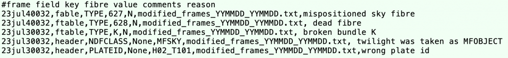
frame: name of frames to be modified
field: ftable or header
key: keyword to be modified
fibre: Either fibre numeric id or bundle name. When modifying the header (field=header), this should be None.
value: new values for the key
comments: comments come into the header
reason: description for the DR team
From the above example, the first line will change the type of fibre 627 as N. The third will change the type of whole fibres of bundle K as N. The fourth will change the NDFCLASS of the frame as MFSKY. The fifth will change the tile name (PLATEID) of the frame.
c. run the Hector manager
Important: Confirm that no instances of the Hector manager are currently active before starting a new session.
Then start the manager.
In [1]: import hector             # this imports the *hector* package
In [2]: mngr=hector.manager.Manager("YYMMDD_YYMMDD", fast=True, n_cpu=20)
As the manager runs, it will process the specified file, and you should see confirmation messages, such as:
Adding file:  05nov30017.fits ...
  Change the TYPE of all fibre in bundle Q to N
In [3]: exit()
Important: The manager must be properly closed with exit() to ensure the changes are saved permanently.
d. Notification of raw frame modifications
In the observing log, clearly state that you have modified something in the raw frame using the above method. If necessary, contact the DR team to inform them of the modification so they can monitor it during the data reduction process.
Essential: check tramline mapping and spectral focusing
On the first night, once the dome is dark and after the spectrograph has been focused, it is ESSENTIAL to take a dome flat and an arc frame and check the tramline mapping and spectral focus. We are finding frequent failures of tramline mapping, and therefore, it is essential to check the tramline for EVERY SINGLE DOME FLAT in real time. For spectral focusing, we only check the first arc frame of the day.
You should learn how to use check_tramline() in the afternoon on the first day and keep running this function every time you take new dome flat during the night.
In [4]: mngr.import_aat()                         #import new files of the run
In [5]: mngr.make_tlm()                           #tramline mapping using 2dfdr
In [6]: mngr.reduce_arc(check_focus='21oct10002') #check spectral focus for the given arc
In [7]: mngr.reduce_fflat()                       #reduce flat frame
In [8]: mngr.check_tramline()                     #check tramline mapping
                                                  #use date='YYMMDD' to specify date
tramline
You should learn how to use check_tramline() in the afternoon on the first day and keep running this function every time you take new dome flat during the night. Once you run check_tramline(), it generates a text file /data/hector/reduction/YYMMDD_YYMMDD/tlm_failure_YYMMDD_YYMMDD.txt where you can find the list of flat field frames checked for tramline mapping. It also gives you directions that you should follow when it detects any failure in tramline. Specifically, the text file may direct you to check whether the frame is saturated or out of focus which can cause a catastrophic failure in tramline mapping. It may also send you to the top end to check the sky fibre position. It also guides you to visually check tramlines. It may also give you a warning of tramline cutoff which may require to adjust spectrograph mounting.
You may find examples from the data reduction machine:
/home/hector/software/hector/observing/check_tramline_example.pdf
If you confirm any tramline failures that you could not fix, you immediately report this to Sree Oh (sreemario@gmail.com), Madusha Gunawardhana (madusha.gunawardhana@sydney.edu.au), and Scott Croom (scott.croom@sydney.edu.au) and send the raw file (e.g. 29jun40003.fits) and the text file (tlm_failure.txt).
spectral focusing
Reducing arc frame with the ‘check_focus’ option generates diagnostic figures tracking the spectral focus values of the run: /data/hector/reduction/YYMMDD_YYMMDD/qc_plots/
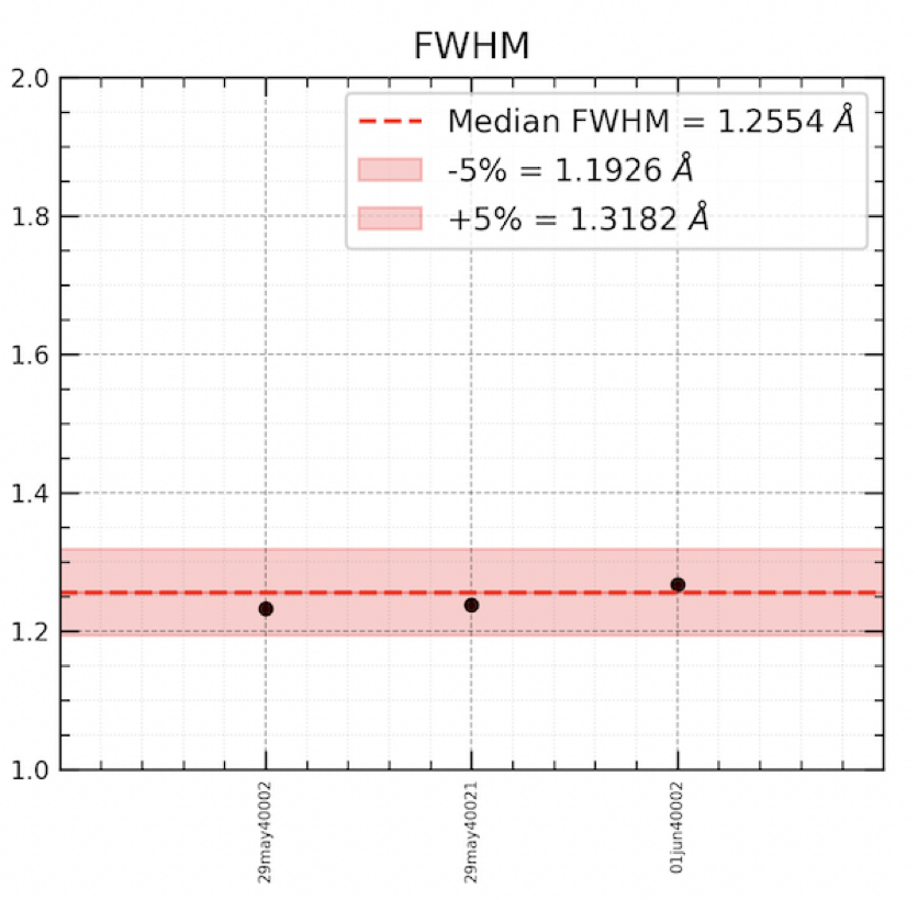
If the FWHM values are off by 5% of the median, consider redoing spectrograph focusing.
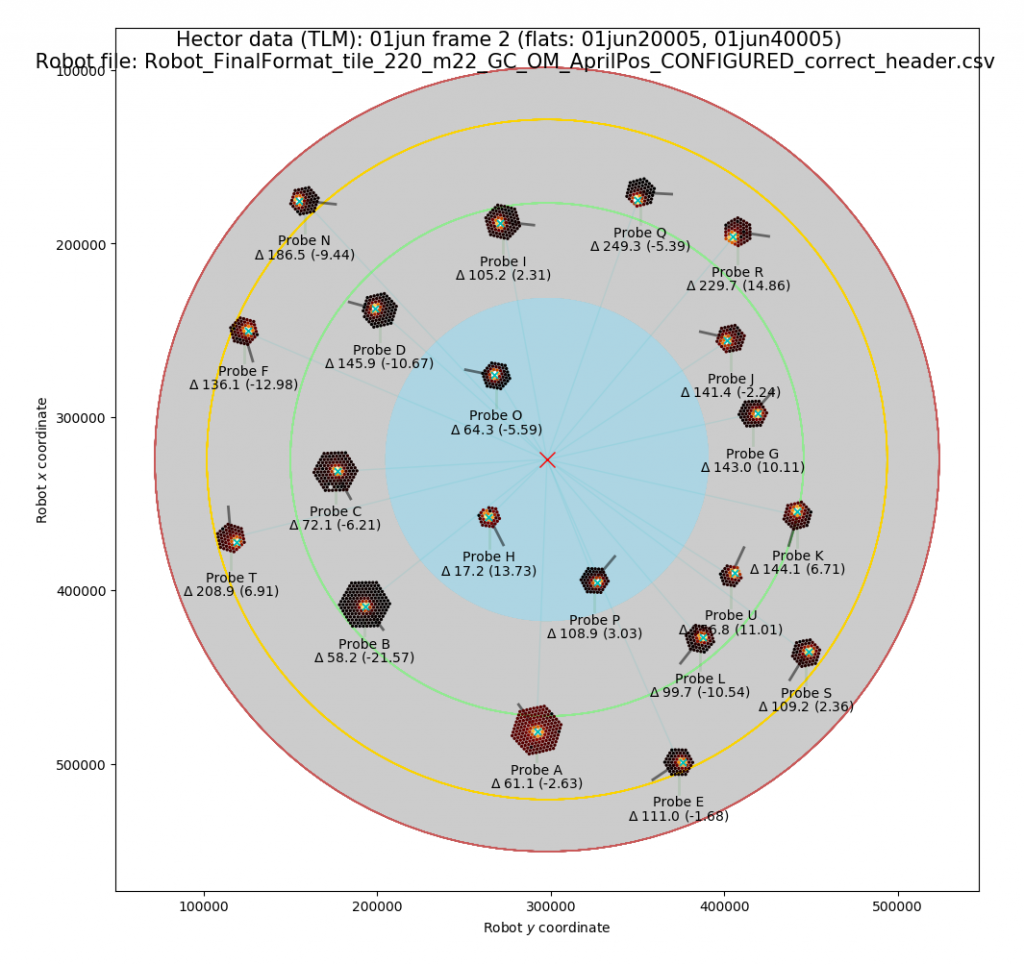
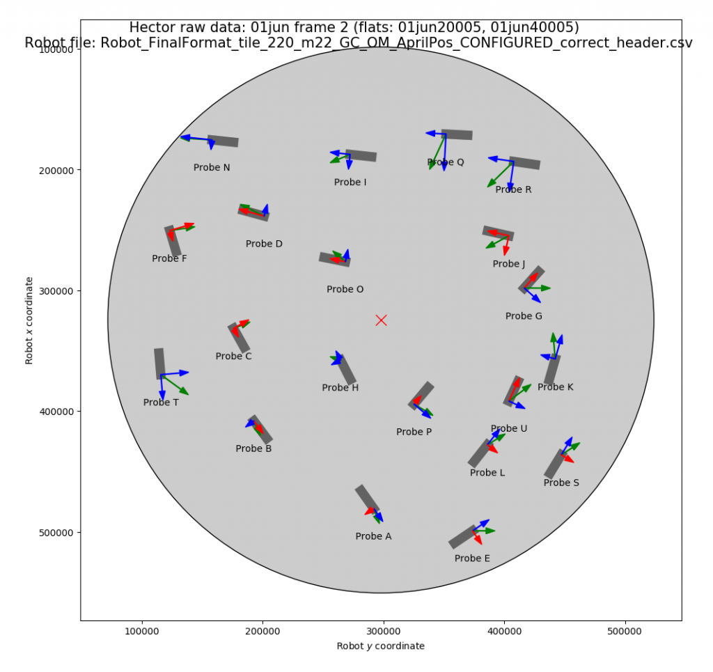
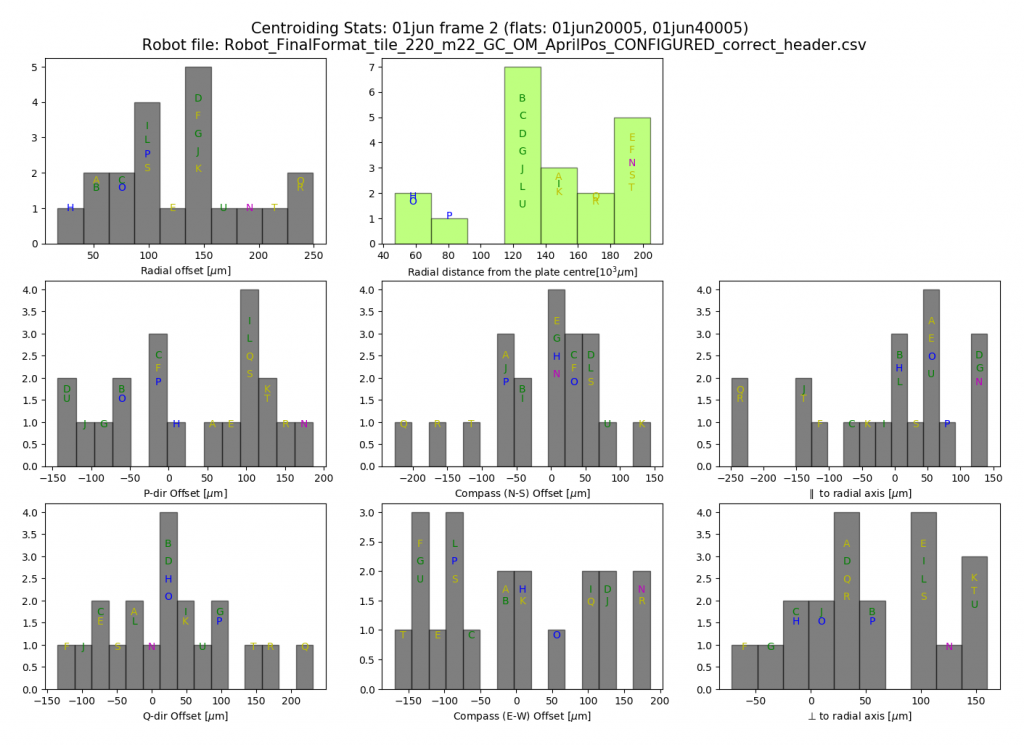
Essential: quick-look plots to check centring
Once the tramline is made (via mngr.make_tlm()) and an object frame is imported (via mngr.import_aat()), you are ready to run the quick-look tool. Note that the quick-look tool and mngr.reduce_arc() can go parallel, and observers do not need to wait until mngr.check_tramline() is done.
The quick-look tool generates the following three plots needed for checking centring.
Instructions on setting up and running the quick-look tool
The quick-look tool access the working data directory you create when you run the Hector manager on the first day of the observing run, i.e. a directory of the name “YYMMDD_YYMMDD” of the current observing run.
On the first day:
In a separate terminal navigate to the /home/hector/software/hector/observing/Quick_Look_Tools/ folder.
– open an ipython shell, and type:
run update_quick_look_config.py –observing_run_dates[the name of the working directory]
Example:

This sets up the directory structure within the quick-look tool, and you only need to run this command once.
Both the robot and tile files for the field should be in the raw data directory under the current run date.
How to run the quick-look tool:
Once you set up the directory structure, you are ready run the quick-look script. To run this script, you need to provide the following:
- Object frame run number
- Partially reduced flat frame run number (it is the *tlm.fits file that the code looks for)
- File prefix (e.g. 28jun, 14mar, etc.)
- Robot file name (only need to provide the robot file name, but both the robot and tile files should be in the raw data directory under the current run date)
In Ipyton shell type:
run display_probes.py [object run number] [flat run number] –file_prefix [file prefix] –robot_file_name [robot file name]
Example:
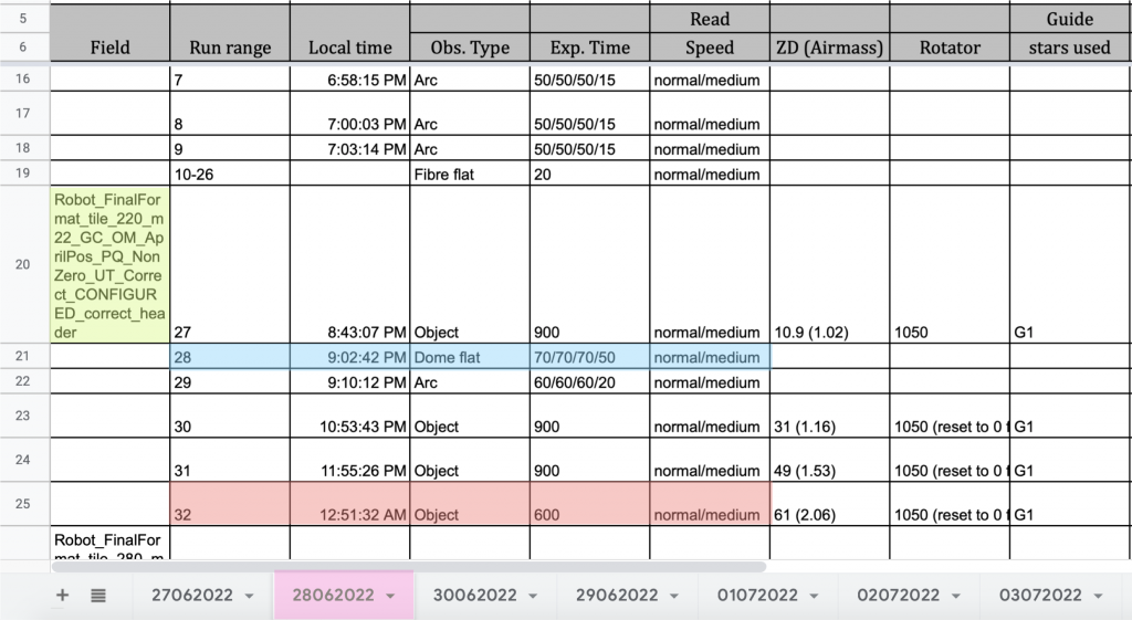
Above is a screenshot of the observations taken on 28 June 2022 (highlighted in magenta). To generate the quick-look plots for the object run number 32 (highlighted in red) using its flat (run 28; highlighted blue) and the robot file, you need to run the following command.
In Ipython:
run display_probes.py 32 28 --file_prefix 28jun --robot_file_name Robot__A3376_T033.csv
Once the quick-look tool starts to run, the terminal will display some information relevant to the data/flat frames given. This is your chance to check whether the quick-look tool uses the correct data and flat frames across all CCDs. The terminal output will look like:
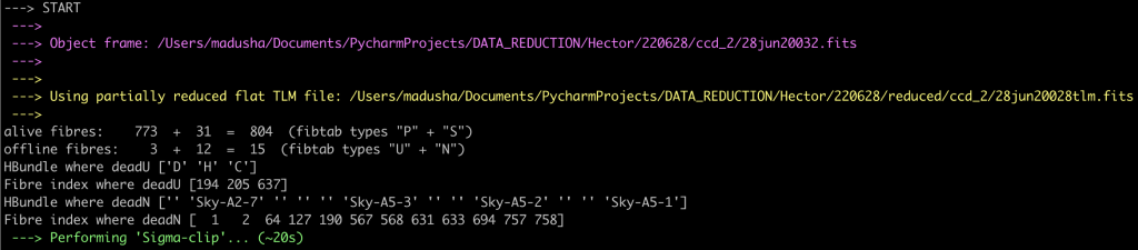
The colour-coded lines provide information on the inputted data/flat frames.
Then the tool will start centroid-fitting…
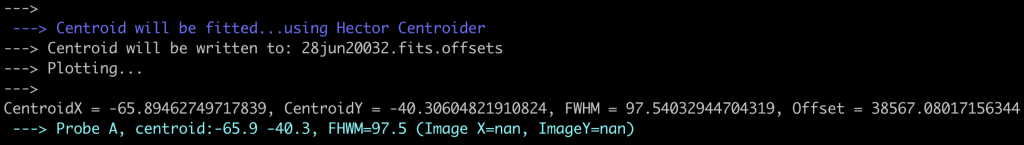
The quick-look script doesn’t run to completion without user input. You will be asked to provide some feedback on the centroid fits.
At this stage, examine the figure that the quick-look tool has produced and exclude any hexabundles with incorrect centroid fits.
All outputs from the quick-look tool are saved in the “Outputs” folder under the working data directory.
Changing the default running mode of the quick-look tool
There are several keywords that you can use to change the default running mode of the quick-look tool. Some keywords can be invoked directly when running the quick-look tool, and some via the “update_quick_look_config.py” script.
IMPORTANT: keywords invoked via the “update_quick_look_config.py” script will be added permantly to the quick-look configuration file, whereas the keywords invoked when running the quick-look tool applies only to that instance.
Table 1: A list of available keywords
| Keyword | Can be invoked when running the quick-look tool* | Can be invoked prior to running the quick-look tool (i.e., in the “”update_quick_look_config” script)** | Example |
| –file_prefix | yes | yes | –file_prefix 28jun |
| –robot_file_name | yes | yes | –robot_file_name Robot_FinalFormat_etc |
| –spectrograph_not_used | yes | yes | –spectrograph_not_used AAOmega |
| –red_or_blue | yes | yes | –red_or_blue red |
| –sigma_clip | No | Yes | –sigma_clip True |
| –centroid | No | Yes | –centroid True |
* the change applies only to that instance of the quick-look tool
** permanently adds the keyword to the quick-look configuration file.
Table 2: Descriptions of the keywords
| Keyword | Explanation |
| –file_prefix | the data prefix appended to the raw data frames |
| –robot_file_name | the name of the robot file |
| –spectrograph_not_used | Specify which spectrograph to remove from the analysis (options: AAOmega, Hector, None). By default set to None |
| –red_or_blue | Specify which arm to use for the analysis (options: red, blue, both), By default set to ‘both’ |
| –sigma_clip | Specify whether to perform sigma clipping on the data (options: True, False). By default set to True |
| –centroid | Specify whether to perform centroiding (options: True, False). By default set to True |
Essential: QC summary
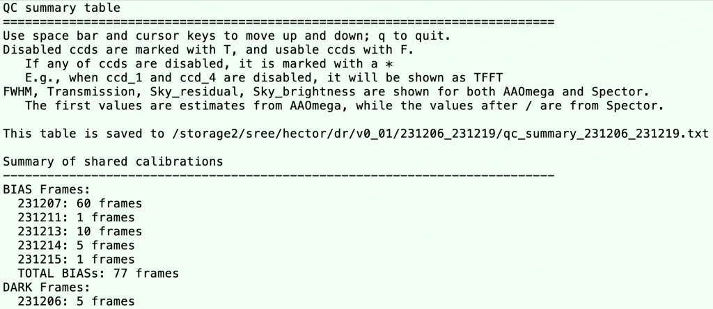
At any time you can print out a summary of the frames observed, including some basic quality control metrics:
In [4]: mngr.qc_summary() #this will print out summary of the frames
It also generates a text file named /data/hector/reduction/YYMMDD_YYMMDD/qc_summary_YYMMDD_YYMMDD.txt
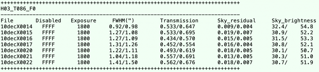
The QC values are not filled in until certain steps of the data reduction have been done. After the mngr.telluric_correct(), it starts to show seeing (FWHM “). You need to get as far as mngr.scale_frames() to see transmission. While observing, keep an eye on the seeing and the transmission. If the seeing is above 3″ or the transmission is below about 0.7, the data are unlikely to be of much use. If so, plan to re-take the frame.
If the seeing from both instruments are above 3″ or both transmissions are below about 0.33, the data are unlikely to be of much use. If so, plan to re-take the frame.
The minimum requirement for cubing is to have at least 6 dithered frames with exposure times greater than 1600s. If observers are short on time, they may need to decide to reduce the exposure time for the last dithers or skip the last one.
Essential: upload raw data to the data central cloud
It is extremely important to upload the raw data to the data central cloud. Note that the data at AAT machines are cleaned up regularly. Do not wait until the last day, and observers upload data daily basis.
Every night, when the observing is getting to the end, observers upload raw data from the reduction machine. On the last night, observers should double check that all the frames have been loaded to the reduction machine, before uploading.
In [1]: mngr.import_aat()
In [2]: exit
(base) hector@aatlxe:~$ rsync -avhPin -e 'ssh -p 2232' --exclude 'reduced' /data/hector/reduction/YYMMDD_YYMMDD hector@uploads.datacentral.org.au:/data/Observing/20YYMMDD_20YYMMDD/
L3tMe!nPle@se
The above with the ‘n’ flag prints the list of frames to be uploaded, but it does not actually transfer any frames. Once the list has been confirmed, upload data to the data central, without using the ‘n’ flag.
(base) hector@aatlxe:~$ rsync -avhPi -e 'ssh -p 2232' --exclude 'reduced' /data/hector/reduction/YYMMDD_YYMMDD hector@uploads.datacentral.org.au:/data/Observing/20YYMMDD_20YYMMDD/
The rsync (or scp) is recommended but if it doesn’t work, observers may drag and drop the ‘raw’ folder from the reduction machine to the data central cloud. Navigate to Hector/Observing/20YYMMDD_20YYMMDD/ and generate a folder named “YYMMDD_YYMMDD‘’ using the + button. Then, come into the folder and drag and drop /data/hector/reduction/YYMMDD_YYMMDD/raw there. Also, don’t forget to upload all txt files from YYMMDD_YYMMDD
It is possible (or extremely likely!) that the browser will give weird errors. If so, reload it and consider copying one folder at the time. This should not be done on the last day, but at the end of every night given how temperamental can be the system. You may double check the size of uploaded and local data to make sure you uploaded all the raw data. Don’t forget to upload daytime calibration frames.
Essential: upload log on the Hector wiki
At the end of the run, please upload the log to the Hector wiki at https://hector.survey.org.au/wiki/observing/observing-summary. This is important for other team members to understand what happened during observing. Download the log Excel file via File-Download- Excel file. At the end-left of the wiki page you need to click the “Edit” bottom, you need to create a new Header specifying the number of the run, the dates, the observers. Then, add the downloaded Excel file as a “File” block. Have a look at this video on how to edit wiki pages https://hector.survey.org.au/wiki/wiki-help. If you have any issue, please contact Stefania Barsanti (stefania.barsanti@anu.edu.au)
If you take any calibration frames, please list them at this page: https://hector.survey.org.au/wiki/calibration-frames.
Night-time Calibration Frames (Flats, Arcs, Twilights)
There are calibration frames to be taken every night, often more than once per night.
Flats
When observing a 7-point dither on galaxies, the aim is to take a flat and arc in the middle of the dither frames (after the 3rd or 4th dither) then continue on with the dithers. The 7-point dither script automatically does the flat and arc in the middle of the 7 exposures. When the script is run (see below – observing galaxies ) it will request the exposure times for the flat and arc.
Flat fields are images taken with uniform illimitation across every hexabundle and sky fibre. The allow the data reduction software to trace out the position of each fibre on the CCD and correct for fibre-to-fibre throughput variations. There are three different types of flat field frames: twilight flat, flap flats and dome flats.
The best possible flat-fields to use are twilight flats. Taking twilight flats is therefore a very high priority at the start and end of every night.
When observing twilight flats follow this procedure:
- Point the telescope about 1 hr away from zenith in the direction opposite the sun (i.e. 1 hr E at dusk or 1 hr W at dawn). This is the “flattest” part of the sky, according to lore.
- On the CCD control, select “Offset Sky” as the observation type. Do not select twilight flat!
- If it is dusk, start within 30 sec after sunset with a ~5s exposure
- You may give half exposures for CCD4 to safely avoid saturation
- When the frame has read out check the counts in various parts of the frame. 30,000 – 40,000 are good numbers for the highest values. Less than 10,000 or greater than 55,000 is not great.
- Offset the telescope between frames by 60″ in a random direction (just to ensure that if you happen to land on a star not all your twilights will be affected).
- For the next frame double your exposure time if the counts were good, or scale that up or down to improve the counts.
- Aim to keep the counts constant-ish between twilight frames. This isn’t too critical so don’t worry, just note down in the log if you saturate one or if one has too few counts. The latter may still be useful (the former should never be used).
- Remember, you only have about 15 minutes of useful time here, so keep taking frames, doubling the time for each exposure and offsetting the telescope between exposures, until you get to about 200sec. Once you need much longer than 200sec, the sky is too dark.
- If observing dawn twilights, reverse the procedure, starting with your longest exposure about 15 mins before sunrise and cutting your exposures accordingly as the sun rises.
Dome flats are observed by pointing the telescope at a screen next to the dome opening and illuminating it with LED lights arranged around the top-end. The spectral and spatial flatness of the dome flats was not ideal at the start of Hector but has been improved with the addition of new lamps (July 2022). The current advice is to take Dome Flats for each exposure as well as twilight flats when possible.
To take a Dome Flat (Essential) when not part of a 7-point dither sequence:
Try to take a dome flat at the position of the field. Ignore the warning about the “old” dome screen – it has been repainted and both dome screens are now actually “new”.
- Check that a position is entered into the Position (J2000) box of the Telescope Control dialogue box (e.g. see below). If not, load a Hector Config and Robot file at the bottom of the CCD control dialogue box and click “Load positions from HECTOR file to input fields” in the telescope control task. If a field isn’t loaded correctly then the dome flat routine will offset the telescope AWAY from the flat field screen! Double check the alignment between the screen and telescope pointing. The night assistant may tell you whether the screen is well loaded or not.
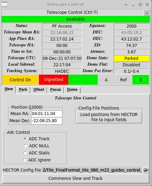
- If the telescope is at a greater ZD than 60 degrees, then the dome screen will not move to a position that is aligned with the telescope. Instead move the telescope up a bit away from the field so it is at ZD< 60 deg and take the flat there. But also double check the engagement of the screen. If not engaged, request the night assistant to make the telescope track any nearby object.
- Select “Fibre Flat” from the CCD control task.
- Select “Dome Flat” from the available options.
- Use an exposure time of 60/60/50/25 seconds for four spectrographs. Aiming for 30,000-40,000 counts at the peaks.
To take a Flap Flat (Not normally used because tramlines unreliable – only for testing light into fibres):
- Select “Fibre Flat” from the CCD control task
- Select the 75W AAOmega lamp (which is the default option)
- For Spector in the medium readout mode, use an exposure time of 20 seconds for the blue arm (HBL) and 10 seconds for the red arm (HRD). Use 20 seconds for both arms of AAOmega. Selecting 20 seconds for the Spector red arm will saturate it!
- If taking multiple flats in a row, you can tick the “Leave the lamps and flats in position” dialogue box.
- Check that the observation has 30-40,000 counts at the far end of both red CCDs.
Arc frames
Arc frames are observations of the emission spectrum from one or more arc lamps. They allow the data reduction software to calibrate the wavelength solution across the CCD.
To take an arc frame:
- Select “Arc” from the CCD control panel.
- Select the CuAr1, CuAr2, Helium 1, FeAr1 and FeAr2 lamps from the dialogue box.
- For Spector in ‘medium’ readout mode, use an exposure time of 80/80/80/20 seconds for AAOmega and Spector.
Focussing the Telescope
Telescope focus must be checked every night during twilight and therefore does not take up science time (unless of course twilight is clouded out!). It must also be rechecked after every plate change. Focus should not change much from night to night, unless there has been a large temperature change. For a decent starting point on the first night, go to the focus position recorded during the last Hector run.
We must recheck the focus after every plate change since the telescope must be removed from computer control when we’re working at the top end. The process of changing the plate may slightly change the telescope focus drive, which would usually automatically move back to its desired value. When we’re working at the top end, however, this tuning may cause an unexpected noise which could conceivably lead to an accident. The AAT staff have therefore been advised to stop the telescope’s automatic focus control whilst the plate is being changed, and so the focus is not guaranteed to remain at the value set previously during the night.
The telescope is focussed using the guide bundles. On the guide bundle plot readout, select the “FWHM” to be plotted and unselect the “intensity”. In the telescope control dialog box, the telescope focus can be adjusted in the “focus” tab. Move the focus in steps of 0.2 and watch the FWHM plot. After each change give it some time for the plot to settle down. Step through focus and out both sides until the best focus is identified, which is the when the FWHM plot is at a minimum.
Measuring and Correcting the Global Plate Rotation
A plate rotator on the Hector plate can adjust the rotation of the plate by +/-1000 millideg.
To adjust the rotation, set the rotator to 0 millidegrees then back to the required value. As at Feb 2022, the small steps on the rotator are not reliable. In the meantime, between each 30 minute exposure, the rotation should be checked and recentred.
Before beginning a dither sequence, check the rotation, the rotation can be adjusted to best centre all guide bundles in the guider. Details given below in “Observing Galaxies”.
Spectrophotometric Standards
Once or (better) twice per night you should observe spectrophotometric standards from the list below.
Sree (29 Feb 2024):
Do not observe the following primary standard stars: CD-34d241, EG21, LTT4364, LTT4816, HR7950, HR7596, HR4963
You can observe the following primary standard stars for lower priority, but should also observe other standard stars not listed here: LTT9239, LTT1788, LTT7987, LTT3864
| Object | RA(J2000) | Dec(J2000) | PM dRA | PM dDec | mag | Type/comment |
DR: No high resolution spec | ||||||
DR: No high resolution spec | ||||||
| **LTT1788 | 03 48 22.17 | -39 08 33.6 | 250 | -210 | 13.16 | F |
| GD50 | 03 48 50.06 | -00 58 30.4 | 64 | -161 | 14.06 | DA2 |
| SA95-42 | 03 53 43.67 | -00 04 33.0 | -20 | -98 | 15.61 | DA |
| LTT3218 | 08 41 32.37 | -32 56 32.9 | -1100 | 1340 | 11.86 | DA 100s gives peak of ~ 2000 counts in red. High proper motion. Can be missed in the bundle if you don’t take the proper motion into account (alternatively drive from main telescope control). |
| **LTT3864 | 10 32 13.90 | -35 37 42.4 | -263.7 | -8.0 | 12.17 | F – 100s gives peak of ~ 1200/1000 counts in blue/red |
DR: No high resolution spec | ||||||
DR: No high resolution spec | ||||||
| G60-54 | 13 00 09.53 | +03 28 55.7 | -428 | -870 | 15.81 | DC |
DR: Too bright. Moffat fitting fails | ||||||
| CD-32d9927 | 14 11 46.37 | -33 03 14.3 | -6.5 | 4.1 | 10.42 | A0 |
| LTT6248 | 15 39 00.02 | -28 35 33.1 | -233.3 | -175.2 | 11.80 | A |
| EG274 | 16 23 33.75 | -39 13 47.5 | 76.19 | 0.96 | 11.03 | DA (120 sec gives ~4000 counts in good seeing) |
| A0III bright, needs ~5sec exposure. DR: Too bright. Moffat fitting fails | ||||||
| **LTT7987 | 20 10 57.38 | -30 13 01.2 | -344.45 | -250.60 | 12.23 | DA (wasn’t able to find this one 14-Aug-15?) |
| G24-9 | 20 13 56.05 | +06 42 55.2 | -250 | -578 | 15.72 | DC |
DR: Too bright. Moffat fitting fails | ||||||
| G93-48 | 21 52 25.33 | +02 23 24.3 | 20.25 | -304.55 | 12.74 | DA3 |
| **LTT9239 | 22 52 40.88 | -20 35 26.3 | 80.6 | -309.0 | 12.07 | F |
| LTT9491 | 23 19 34.98 | -17 05 29.8 | 270 | 0 | 14.11 | DC |
Steps 1 – 5 below are currently (July 2022) NOT being used! They will be implemented in the coming months and so are being left in the manual for now. Skip to “July 2022: Standard Stars” section
To observe a standard star, there is a very nice tool to do this. Invoke it with the “Commands->Do Standard Star”
A new dialog pops up. It is in the style of a wizard – it walks you through what is required.
- Select the guide bundle you want to use from a drop down guide bundles used in the configuration.
- Select the IFU you what to use from the drop-down. Both guide bundles and IFUs are listed in order of distance from the center, closest first. AS you will be doing standard star observations in at least 2 hexabundles, start with the closest one. Avoid using low thput hexabundles: E, F, H
- Enter the standard star position and name (the name is used for the headers). Press “Calculate”. Note – before doing the standard star slew, the position is checked to make sure the dome flat field position can be reached (for about 1 hour). Note that the offsets that appear onscreen are not the direct offsets of the telescope and are not expected to agree with the output of the old python program.
- Work through the “Operations” at the bottom of the window.
- Slew to star
- Apply “Field Center to Guide Bundle offset”
- Have night assistant center on the guide bundle.
- Apply “Guide bundle to IFU offset”
- “Run the observing script.” The script will prompt for an exposure time. The script will take three flux calibration exposures (with offsets of 2.5 arc-seconds in first RA and then Dec between exposures). It will then take a FLAT and an ARC using standard exposure times in the script (80 seconds and 10 seconds) including moving the dome windscreen to the correct position and turning on/off the lamps.
If for some reason the default 10 and 80s exposure times for the arc and flat are not giving the correct counts, then these can be changed by editing the script, but do not edit any other part of the script apart from the ftime and atime values for flat and arc respectively in
~/obsscripts/sami/sami_std_star_data_acq.obsscript
“5.” You then need to observe the standard through a second hexabundle. To do so you can remove the IFU to Guide offset and then select a new IFU and repeat the above procedure.
HERE are the old instructions for observing standard stars, which will stay here until the new tool is tested, but these have been superseded by the above tool: You must get it into a hexabundle! The procedure is:
- Point the telescope directly at the star.
- Offset the telescope to put the star into a guide bundle.
- Acquire and guide off the star for a moment, to ensure it is stable and in the centre of the guide bundle.
- Offset the telescope to put the star into a hexabundle. Take an observation. This observation may not be perfectly centred in the hexabundle but that is OK as 2-3 position offsets are required.
- Offset the telescope to centre the star in the hexabundle, then take the second image. If there is time, do 1 further offset of about 2-3″ in any direction and take a third image.
- Reverse the telescope offset, to put the star back in the guide bundle, then do a new offset to a different hexabundle and repeat the procedure of 2-3 images with offsets within the hexabundle.
- Take a dome flat and arc in the field position. Make a note in the log to show that these were taken at the position of the standard star.
The correct offset distances are calculated by entering:
In [1]: sami.utils.other.offset_hexa(‘path/to/csv/file.csv’)
The CSV file path should point to the allocation CSV file that describes the current plugging. It will output something like:
———————————————————————-
Move the telescope 192.26 arcsec W and 465.29 arcsec S
The star will move from the central hole
to guider 1 (G1 on plate)
Move the telescope 45.43 arcsec W and 268.23 arcsec S
The star will move from guider 1 (G1 on plate)
to object probe 6 (P6 on plate)
———————————————————————-
Ask the night assistant to jog the telescope by the specified amounts. By default the offset_hexa function will select the probes closest to the centre. To override this you can specify which guide and/or object probes to use by entering them as keywords, using the numbers on the plate:
In [1]: sami.utils.other.offset_hexa(‘path/to/csv/file.csv’, guide=2, obj=7)
If for some reason you need to skip the guide bundle and move straight to the hexabundle, specify guide=’skip’.
July 2022: Standard Stars
Once per field you should observe spectrophotometric standards from the list shown earlier.
The Hector Offsets script
A useful tool during standard star observations is the Hector_Offsets script. To use it, type a command of the following form into the terminal:
$ cd ~/software/hector/observing/
$ ./Hector_Offsets /path/to/Tile/file location_1 location_2
Or
$ ipython Hector_Offsets /path…
This will output the necessary offsets which you should apply to the telescope (I.e. to read out to the night assistant) to move the star from “location_1” to “location_2”. The values for “location” can be:
- “centre”, corresponding to the field plate centre
- “GS1” to “GS6”, corresponding to the guide bundles 1 – 6
- “A” to “U”, corresponding to each of the Hexabundles
So, to calculate the required offsets to move from the plate centre to guide bundle 3, use:
$ ./Hector_Offsets /path/to/Tile/file centre GS3
Standard Star Procedure
- Find a standard star from the lists mentioned above. Give the coordinates of the standard star to the night assistant and slew the telescope. The centre of the field plate should now be pointing at the star.
- The Hector_Offsets script is in the hector python package, e.g. /hector/software/hector/observing/Hector_Offsets – make sure you are using this version.
- Use Hector_Offsets to find the offsets you should apply to the telescope to put the standard star into a guide bundle (e.g. in this example we use guide bundle 1, but you should pick one close to the centre):
$ ./Hector_Offsets /path/to/Tile/file centre GS1
Get the night assistant to apply these offsets and ensure that you see the star in the correct bundle. Guide from just this bundle for 5-10 seconds to make sure everything is stable and settled.
If you prefer you can now offset the telescope yourself. In a terminal, type drama, then;
- offset 3 5
- – adds a relative offset of 3 arcseconds east and 5 arcseconds north,
- – adds a relative offset of 3 arcseconds east and 5 arcseconds north,
- offset -3 -2
- – adds a relative offset of 3 arcseconds west, 2 arcseconds south.
- set-base-here
- – marks the current position as new base.
- – marks the current position as new base.
- centre
- – moves to the base position
- – moves to the base position
- show-offset
- -displays the telescope offset from base in arc seconds (east, north)
- Next, offset the telescope to move the star from this guide bundle to a Hexabundle. Try and pick one nearby. Hexabundles A, B and C are slightly larger than the rest so make a good choice. Also avoid using low throughput hexabundles: E, F, H
$ ./Hector_Offsets /path/to/Tile/file GS1 A
- Take an exposure and use the quick look tool to see how well centred the star is. It doesn’t have to be perfectly in the middle, since we need 2-3 dithered exposures of the star. Just make sure it’s not falling off the edge of the bundle.
- Offset the telescope to centre the star and take a second exposure.
- If there is time, offset the telescope 2-3″ in any direction and take a third exposure.
- Reverse the telescope offset, to put the star back in the guide bundle, then do a new offset to a different hexabundle. Make sure that this second hexabundle feeds the other spectrograph to the one you’ve just done! For example, if the first observation was in Hexabundle A, which feeds AAOmega, take an observation in one of the Spector hexabundles (I through to U). Repeat the procedure of 2-3 images with offsets within the hexabundle.
- Take a dome flat and arc in the field position. Make a note in the log to show that these were taken at the position of the standard star.
Observing Galaxies
Guiding and field rotation
Before starting an observation the guiding and field rotation must be set.
- The Hector guider instructions can be found <here – add link> but a summary is given now.
- Set the Reciprocal feedback to 5 and start with an exposure time of 1sec.
- First set the rotator to a reasonable guestimate (e.g. the last used value, or ~ 1050millideg), otherwise if it is at zero then no stars may be in their guide bundles.
- If there any issue with any of the guide bundles (e.g. star position was clearly wrong for one) then from the TV Guider window “Guider” menu -> Guider configuration -> a box pops up listing the guide stars. Deselect that guide bundle.
- Select “guide centre”. Not all stars may be centred in their guide bundles at the same time. The higher the airmass, the more this will be the case.
- Now, adjust the rotator by setting “0” then setting the value of rotation required. (if you do not go to 0 between changing the settings then the rotator will not rotate). Change the rotator until all the stars in the guide bundles are as well centred to the crosses as they can be. Select the “2dF guide plot” tab on the guider and the dots in their circles should be along a virtual line from the centre of the plot, and this gives an indication of whether rotating the field will better centre the dots.The best strategy is to adjust the rotation in steps of 20 millidegrees from about 1020 to about 1080 to see when the positioning clearly goes off at either ends of the range, then in the centre of the range there will be several values with little difference in the rotator settings, so you need to go out beyond those in order to find the midpoint where the rotation is best fit. Note that 20millideg is a change of about 100 microns (or 1 fibre core) at the edge of the plate, so we aim to get this right to within 20millideg if possible. If the sky conditions are poor then that may not be possible. NOTE : don’t spend too much time because the rotation will be confirmed (and adjusted) in the next step with the Acquisition image.
- Take a 300 sec acquisition image and adjust the rotation if the two secondary standards (in hexabundles U and H) are not well into their bundles (if they are on the edge then the dither pattern will lose them in some exposures and the data cannot be used without these stars – U and H MUST have stars in their bundles.).
- Generate the Quick look image. Plot the histogram after the quick look image and check the rotation on lower right histogram (“perpendicular to radius” histogram) and see how many microns would put the zero roughly in the centre of the distribution (ignoring outliers which will be diffuse/blobby galaxies). Based on the number of microns to centre the distribution and where the bundles are on the plate (Top centre histogram), use the rule of 20 millideg rotation is 100um at the edge of the plate, and a larger number of millideg rotates the plate clockwise (objects move anticlockwise) on the plate view.
Once the rotation is correct then select all the good guide bundles to be guided on and once the guiding with “guide centre” has brought them all as close as possible to the centres of their bundles then select “guide here”.
Then continue to a science exposure.
Galaxy fields are observed in a fixed, seven-point dither pattern by script ‘hector_dither’. The script does the following:
- Observe four of the seven 1800-second galaxy exposures.
- Observe an arc.
- Observe a field-position dome flat.
- Observe the remaining two 1800-second galaxy exposures.
To run the script, in the HECTOR CCD control dialog, select the folder icon to the right of ‘Scripts:’ below the ‘Start CCD Run’ button. Select the ‘hector_dither’ script and ‘Continue’. Click on ‘Run Script’ and then follow the prompts to enter the object exposure time, and then asks if you want to do a flat and arc between the 4th and 5th dither and usually you should do that (hence accept the default) but if you are going to take a flat and arc before and after the dither instead then put “1” to stop the script from doing a flat and arc. The exposure times for the flat and arc are coded in the script as 80/80/80/20 (arc) and 60/60/50/25 (flat).
To exit the script early (e.g. if the task crashes), on the HECTOR Hexabundle IFU Control Task, go to ‘Commands’ then ‘Unlock Script’.
To intentionally stop the script (e.g. if cloud has come in) then “Abort run” and it will stop the current exposure and pause the script. Before restarting the script later, ‘skip back’ until the box in the scripts says “Next Cmd:GUIDER_OFFSET ……..” [then the E/W and N/S offset values] because that is the last offset that set up the dither position that was just aborted. That offset will need to be run again to set up the same dither position to continue the script in the future. Then “cont script” from there. Note that you can check the dither values listed in that command match the dither pointing you think you are up to by comparing to the table below.
For reference, the pointing positions are:
| Pointing | Skip to Script line # | Arcsecs [N/S,E/W] |
| (A) | 14 | [0.0, 0.0] |
| (B) | 18 | [0.4N, 0.6W] |
| (C) | 22 | [0.7S, 0.0] |
| (D) | 26 | [0.4N, 0.6E] |
| (E) | 37 | [0.4S, 0.6W] (Start at GUIDER THAW message or guiding may remain frozen from calibration frames) |
| (F) | 44 | [0.4S, 0.6E] |
| (G) | 48 | [0.7N, 0.0] |
Do not “hold” or pause an exposure – it will crash the CCDs.
If the dither pattern needs to be started mid-way through – e.g. if several dithers were done on one night and the remaining dithers need to be done on the next night. Then run the dither script from the beginning, but when it asks “are you ready to continue?” then don’t continue, pause the script and then hit the “skip fwd” button to skip forward until you get to the guide offset command that will set the right offset or the dither you are up to.
E.g. if you need to start form the 2nd (“B”) dither frame then skip ahead past the first guide offset comment and the fits command and the object command and then start running the script at the next guide command because this will set the guide mark in the right place for the second offset before going ahead and taking the offset.
Note that the guide offset positions are shown on the guider in the Dither RA and Dec boxes. Those offsets should match the table above.
Day-time Calibrations (Biases, Darks and Long-slit Flats)
In addition to night-time calibrations, some calibration frames must be taken during the day. These are biases, darks and long-slit flats. You do not need any of these to start observing on the first night, these can be taken during subsequent afternoons. On the first afternoon you should prioritise taking and reducing a working flat and arc.
Before leaving any calibration frames going at the end of the night (while you sleep) you must stop and null the ADC first.
Biases and Darks
Biases are 0s exposures to provide the bias level of the CCDs. We must observe about 50 of these per run. Because the only overhead associated with a bias is read-out time (2 minutes per frame for science observations), observing 50 biases takes only 100 minutes per run. This best done during the afternoon (not the first afternoon), after you have plugged the plate and focussed the spectrograph and before you go on-sky. The AAOmega dark slides should be down (closed) for these frames, so these frames can be done earlier in the day if needs be. You might need 2-3 afternoons to complete this task, because there will be other things to do, but not much more than that!
Darks are exposure-time-matched frames to subtract the dark current from the science frames. Usually with Hector you will use only one or two different exposure times for your galaxy frames. Again, the AAOmega dark slides must be down (closed) when observing darks. Because in normal survey operations the usual exposure time for galaxy frames is 1800s, darks take significantly longer to observe than biases. We must observe 25-30 per run. The best time for darks is after a night’s observing. Set a series of 10-ish running before you go to bed, leaving a note on aatliu to the effect that you are still using the spectrograph. (Note – Your darks might be cut short if people need to work in the AAOmega room. This should be rare though.) When you return the next day to get started you will have darks in your data directory from the previous night.
Long-slit Flats
Long-slit flats, also called detector flats or defocussed flats, calibrate pixel-to-pixel QE of the CCDs. We must observe about 30 of these per run. A good time to observe these is during the afternoon. These must be observed after 16:00 – i.e. with the dome lights off. To observe long-slit flats do the following:
- Defocus both the spectrographs by setting AAOmega blue piston value to 4200 and red piston value to 4100 and set the Spector pistons to be 50 each (but first note what they were at so they can be put back after taking the long-slit flats. Do not set the Spector pistons below 50 or above 4000 or they will reach limit stops. Moving pistons ‘Via home’ may recover from this, otherwise a specific procedure (contact Julia or Tom W) is needed to recover control.
- Point at the dome screen. Set the observation type to “Detector Flat”.
- Take a frame with an exposure time of 40/40/40/25 if using the flap lamp. You will be given an option of lamps, select “75W AAOmega” to do a flappy flat. (NOTE: The flats that are used for defocussed flats aim to be have low variation in fibre-to-fibre spectral response. This means the resulting illumination in the defocussed flats is more uniform. As at Feb 2022 the dome flat illumination is still not optimised and is less flat than the flap flat. For now use the flap flat but in the future when the dome flat system is completed with the new lamps it should be flatter).
- In the read-out frame, check that the images of the fibres are washed out. A long-slit flat should have no structure associated with the fibres.
- Check that the exposure time is ok – i.e. the frame is not saturated anywhere and there are significant counts at all places on the detector (a peak of 10,000 is a good guideline).
- Once you are satisfied with your set-up observe a series of these frames – Take 10 exposures at 40/40/40/25, then 10 x 38/38/38/18, then 10 x 35/35/35/15
Troubleshooting
Drama (Hector control software Failure)
If the hector control software (drama) crashes, please go through the following steps.
- First, exit drama, using either clean exit ( ), and if not possible do a dirty shutdown. If neither work, hit the cross at the top-right, and run command cleanup in terminal.
- Next step is to run cleanup, and type hector
- Then: select commands–>initialise to start the Hector software and initialise the CCDs. This sometimes takes a long time, and you may see that Spector is in a warning state during initialisation.
Guider
If the Guider doesn’t start correctly on initialisation and throws an “Unknown Telescope Configuration” error, it’s usually because the guider task is running from a previous instrument at the night assistant’s panel. Close the guide task (File –> Exit –> Yes) and then ask the night assistant to reset any guider tasks running from their machine. Then run Commands –> Reset –> Recover from the main Hector control task. The guider software should reappear and start correctly. Note that you must close the guider software before doing the reset/recover.
ADC Timeout
When recovering from an ADC timeout, follow these steps
1) “Reset – By Task – ADC”
2) If above fails
3) Go to the 2dF internet power switch page (bookmarked on the building computer under Night Assistant Stuff)
4) Select “Boot” for the ADC and click “Apply”
5) Wait 1 minute
5.5) Exit the guider
6) “Reset – Recover”
Any resetting or task deletion with the PTCS except “Reset – Recover” will
cause the TCS to hang.
Guider not responding to mouse clicks
Workaround next time guider hangs while imaging.
Options -> Tcl Command opens a new Tcl Command Window.
Type enableCaptureButtons and press Apply.
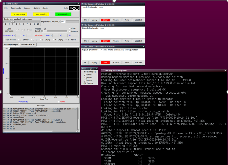
You must then select the ‘Take an Image’ box and then ‘Start Guiding’. Buttons should work normally after this.
At the End of the Night
Ensure the first plate for the following night is configured and ready to go.
It is important that the top end be left with the hexabundles plugged on the plate and the barrel rotated to the observing position. Normally that would be the case but if there have been weather interruptions and that is not the case then plug the plate and rotate the barrel before going to bed because it is NOT safe for site staff to move the telescope with the hexabundles in the holding positions, and the night assistant must put the telescope at zenith to close the mirror covers.
You must stop and null the ADC before leaving any calibrations frames running when you go to bed.
At the End of the Run
On the last night of the run, the instrument change will start at 5am.
Before that time, the last plate must be unplugged with all hexabundles back in their holding positions off the plate on either side, and all sky fibres must be stowed in position zero.
Remove the plate and put it on the robot and start unconfiguring it while the instrument change gets underway. The plate that was on the robot can be put in the Hector room or better still in the cupboard at prime focus that the robot pc monitor site on. Make sure the plate is sitting flat and supported all round.
When the run is over please fill in the AAO’s Observer’s Report Form
Observing checklist below: